Having Fun with Self-Organizing Maps
Introduction
Self-Organizing Maps (SOM), or Kohonen Networks ([1]), is an unsupervised learning method that can be applied to a wide range of problems such as: data visualization, dimensionality reduction or clustering. It was introduced in the 80’ by computer scientist Teuvo Kohonen as a type of neural network ([Kohonen 82],[Kohonen 90]).
In this post we are going to present the basics of the SOM model and build a minimal python implementation based on numpy. It leads to visualizations such as:
There is a huge litterature on SOMs (see [2]), theoretical and applied, this post only aims at having fun with this model over a tiny implementation. The approach is very much inspired by this post ([3]).
We first introduce the maths of the model and then present concrete examples to get more familiar with it.
What’s a SOM ?
For the sake of simplicity we’ll describe SOMs as being supported by a h*w set of 2D points that we call cells, regularly spaced in the plan, also called a point lattice.
We refer to them by assigning them coordinates, here top down in the spirit of numpy matrices.
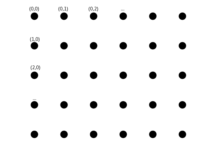
To each of these cells is associated a feature vector of dimension d (d is the same for all cells). In that setting a SOM is entirely described by a h*w matrix containing d dimensional vectors, that is a (h,w,d) tensor.
We thus can construct a zero-initialized SOM with the following code:
1
2
3
4
5
6
7
8
9
10
11
12
13
14
# jdc for step by step class construction
import jdc.jdc as jdc

import numpy as np
import itertools

class SOM(object):
    def __init__(self,h,w,dim_feat):
        """
            Construction of a zero-filled SOM.
            h,w,dim_feat: constructs a (h,w,dim_feat) SOM.
        """
        self.shape = (h,w,dim_feat)
        self.som = np.zeros((h,w,dim_feat))
Note on the code. We construct the code iteratively, the blocks you see are the cells of this notebook.
We use the jdc %%add_to (see [4]) magic command in order to construct the SOM class step by step. If you’re not familiar with notebooks
just consider each of the blocks commencing by %%add_to SOM as updates we do on the class SOM methods.
The entire final code is to be found here.
When a function appears on several blocks such as the __init__ function like here or here it means it has been updated from one block to the other.
Otherwise function calls always refer to the most recent definition of it.
Disclaimer. The code we present could be highly optimized, in particular in its way it interacts with numpy.
What are we going to do with SOMs ?
We are going to train them!!
The idea of a SOM is to feed it with d dimensional data and let it update it’s feature vectors in order to match this data. Furthermore, we want it to group nearby on the lattice data which are originally nearby in the d-dimensional space. This will be done by spreading information in neighbourhoods. This neighbourhood approach concentrate similar data in clusters around close cells on the SOM.
Furthermore, with a SOM we can visualize on a 2D lattice data potentially lying in a very high dimension space. That’s why it can be seen as a dimensionality reduction technique.
All of this being unsupervised as we give our data to the model without additional information.
The best way to have an intuitive understanding of these aspects of SOMs is to code one. Let’s go!!
Finding the Best Matching Unit
At each time step t of the training, we are going to present to the SOM a randomly chosen input vector of our data. Then, we find the cell having the closest (norm L2 speaking) feature vector to that input vector. We call this cell the Best Matching Unit (BMU).
1
2
3
4
5
6
7
8
9
10
11
12
13
14
15
16
17
18
19
20
21
22
23
%%add_to SOM
def train(self,data):
    """
        Training procedure for a SOM.
        data: a N*d matrix, N the number of examples,
              d the same as dim_feat=self.shape[2].
    """
    for t in itertools.count():
        i_data =  np.random.choice(range(len(data)))
        bmu = self.find_bmu(data[i_data])

def find_bmu(self, input_vec):
    """
        Find the BMU of a given input vector.
        input_vec: a d=dim_feat=self.shape[2] input vector.
    """
    list_bmu = []
    for y in range(self.shape[0]):
        for x in range(self.shape[1]):
            dist = np.linalg.norm((input_vec-self.som[y,x]))
            list_bmu.append(((y,x),dist))
    list_bmu.sort(key=lambda x: x[1])
    return list_bmu[0][0]
Updating the BMU
Now that we found the BMU, we want it’s current feature vector \(V_t\) to be closer to the inputed data vector at time t, \(D_t\). Here the update rule we are going to use:
\[V_{t+1} = V_{t} + L(t)*(D_{t}-V_{t})\label{eq:bmu}\]\(L(t)\) is called the learning rate and depends on time t. Remark that if \(L(t) = 1\), we directly replace our feature vector by the input vector. It’s the kind of behavior that we would like to see at the begining of the training but if we want the SOM to “stabilize” we’ll need to decrease L(t) over time. That’s exactly why we define:
\[L(t) = L_0*e^{-\frac{t}{\lambda}} \label{eq:L}\]With \(L_0\) the initial learning rate and \(\lambda\) a time scaling constant.
Let implements these new ideas:
1
2
3
4
5
6
7
8
9
10
11
12
13
14
15
16
17
18
19
20
21
22
23
24
25
26
27
28
29
30
31
32
33
34
35
36
37
38
39
40
41
42
43
44
45
%%add_to SOM
def __init__(self,h,w,dim_feat):
    """
        Construction of a zero-filled SOM.
        h,w,dim_feat: constructs a (h,w,dim_feat) SOM.
    """
    self.shape = (h,w,dim_feat)
    self.som = np.zeros((h,w,dim_feat))

    # Training parameters
    self.L0 = 0.0
    self.lam = 0.0

def train(self,data,L0,lam):
    """
        Training procedure for a SOM.
        data: a N*d matrix, N the number of examples,
              d the same as dim_feat=self.shape[2].
        L0,lam: training parameters.
    """
    self.L0 = L0
    self.lam = lam

    for t in itertools.count():
        i_data =  np.random.choice(range(len(data)))

        bmu = self.find_bmu(data[i_data])
        self.update_bmu(bmu,data[i_data],t)


def update_bmu(self,bmu,input_vector,t):
    """
        Update rule for the BMU.
        bmu: (y,x) BMU's coordinates.
        input_vector: current data vector.
        t: current time.
    """
    self.som[bmu] += self.L(t)*(input_vector-self.som[bmu])

def L(self, t):
    """
        Learning rate formula.
        t: current time.
    """
    return self.L0*np.exp(-t/self.lam)
Updating the rest of the SOM
As suggested before, we are going to communicate the BMU’s update to its neighbourhood. This will lead on having close feature vectors on close cells. That’s why we can see SOMs as a clustering method: it groups together similar information.
Let’s have $W_t$ the feature vector of a cell $\boldsymbol c = (x,y)$, different than the BMU $\boldsymbol c_{0} = (x_0,y_0)$. We are going to update it as below:
\[W_{t+1} = W_{t} + N(\delta,t)*L(t)*(D_{t}-W_{t})\label{eq:non_bmu}\]With $N(\delta,t)$ the neighbouring penalty depending on $\delta = || \boldsymbol c - \boldsymbol c_{0}||_{2}$, the distance between that cell and the BMU, and $t$ the current time.
Indeed, we would like farest cells ($\delta$ high) to be less affected by the BMU’s update. Also, we would like this update to be more and more localized near the BMU over time. As for the learning rate, we want the SOM to “stabilize” over time.
It leads to the following formulation for $N(\delta,t)$:
\[N(\delta,t) = e^{-\frac{\delta^2}{2\sigma(t)^2}}\]Which is a spatial Gaussian decay scaled by radius factor $\sigma(t)$. For the reasons we just mentionned, we want $\sigma(t)$ to get smaller over time so that the “influence area” of the BMU shrinks. We’ll do that in the exact same way as equation $\ref{eq:L}$. It gives:
\[\sigma(t) = \sigma_0 * e^{-\frac{t}{\lambda}}\label{eq:sigma}\]We use the same time scaling $\lambda$ parameter for both $L$ and $\sigma$.
By looking at the update equations $\ref{eq:bmu}$ and $\ref{eq:non_bmu}$ for the BMU cell and non-BMU cells we can notice that the only thing that differs is the $N(\delta,t)$ term. Furthermore, from the BMU to itself $\delta=0$ and gives $N(\delta,t)=1$ which exactly give equation $\ref{eq:bmu}$. Thus we can use equation $\ref{eq:non_bmu}$ as a unique update rule for all cells, BMU and non-BMUs.
Let implements all that:
1
2
3
4
5
6
7
8
9
10
11
12
13
14
15
16
17
18
19
20
21
22
23
24
25
26
27
28
29
30
31
32
33
34
35
36
37
38
39
40
41
42
43
44
45
46
47
48
49
50
51
52
53
54
55
56
57
58
59
60
61
62
63
64
65
66
67
68
69
%%add_to SOM
def __init__(self,h,w,dim_feat):
    """
        Construction of a zero-filled SOM.
        h,w,dim_feat: constructs a (h,w,dim_feat) SOM.
    """
    self.shape = (h,w,dim_feat)
    self.som = np.zeros((h,w,dim_feat))

    # Training parameters
    self.L0 = 0.0
    self.lam = 0.0
    self.sigma0 = 0.0

def train(self,data,L0,lam,sigma0):
    """
        Training procedure for a SOM.
        data: a N*d matrix, N the number of examples,
              d the same as dim_feat=self.shape[2].
        L0,lam,sigma0: training parameters.
    """
    self.L0 = L0
    self.lam = lam
    self.sigma0 = sigma0

    for t in itertools.count():
        i_data =  np.random.choice(range(len(data)))

        bmu = self.find_bmu(data[i_data])
        self.update_som(bmu,data[i_data],t)


def update_som(self,bmu,input_vector,t):
    """
        Calls the update rule on each cell.
        bmu: (y,x) BMU's coordinates.
        input_vector: current data vector.
        t: current time.
    """
    for y in range(self.shape[0]):
        for x in range(self.shape[1]):
            dist_to_bmu = np.linalg.norm((np.array(bmu)-np.array((y,x))))
            self.update_cell((y,x),dist_to_bmu,input_vector,t)

def update_cell(self,cell,dist_to_bmu,input_vector,t):
    """
        Computes the update rule on a cell.
        cell: (y,x) cell's coordinates.
        dist_to_bmu: L2 distance from cell to bmu.
        input_vector: current data vector.
        t: current time.
    """
    self.som[cell] += self.N(dist_to_bmu,t)*self.L(t)*(input_vector-self.som[cell])

def N(self,dist_to_bmu,t):
    """
        Computes the neighbouring penalty.
        dist_to_bmu: L2 distance to bmu.
        t: current time.
    """
    curr_sigma = self.sigma(t)
    return np.exp(-(dist_to_bmu**2)/(2*curr_sigma**2))

def sigma(self, t):
    """
        Neighbouring radius formula.
        t: current time.
    """
    return self.sigma0*np.exp(-t/self.lam)
How to start, how to stop them ?
Two things we have left behind are the begining and the ending of the training procedure.
For the moment we start with a full zero SOM and our train method is an infinite loop.
As often in machine learning, these two stages of the process are foremost a matter of choice.
Initialization
Intuitively it is in our interest to have diversity in our initial SOM so that BMU’s are strong matches and form clusters early. Initialization is a very important part of the SOM process and there’s plenty of options:
- Initialize randomly: uniformly, Gaussian or in any other way. Efficiency will highly depends on our data’s distribution.
- Initialize by sampling: if we have a lot of data compared to the number of cells we can pick some of it randomly to be our initial feature vectors.
Given all these possibilities we are going to leave the choice to the code’s user, implementing a default uniform random initialization in $[0,1]^d$.
In practice we provide the possibility to specify an initializer(h,w,dim_feat) function that returns the initial (h,w,d) SOM tensor:
1
2
3
4
5
6
7
8
9
10
11
12
13
14
15
16
17
18
19
20
21
%%add_to SOM
def train(self,data,L0,lam,sigma0,initializer=np.random.rand):
    """
        Training procedure for a SOM.
        data: a N*d matrix, N the number of examples,
              d the same as dim_feat=self.shape[2].
        L0,lam,sigma0: training parameters.
        initializer: a function taking h,w and dim_feat (*self.shape) as
                     parameters and returning an initial (h,w,dim_feat) tensor.
    """
    self.L0 = L0
    self.lam = lam
    self.sigma0 = sigma0

    self.som = initializer(*self.shape)

    for t in itertools.count():
        i_data =  np.random.choice(range(len(data)))

        bmu = self.find_bmu(data[i_data])
        self.update_som(bmu,data[i_data],t)
Stopping
We choose to stop the process when $\sigma(t) < 1$, that is when updates only concern BMUs and no more significative information spreads on the SOM. Notice that with this criterion, given equation $\ref{eq:sigma}$, we can predict the total training time only with the $\lambda$ and $\sigma_0$ parameters. This gives:
1
2
3
4
5
6
7
8
9
10
11
12
13
14
15
16
17
18
19
20
21
22
23
24
%%add_to SOM
def train(self,data,L0,lam,sigma0,initializer=np.random.rand):
    """
        Training procedure for a SOM.
        data: a N*d matrix, N the number of examples,
              d the same as dim_feat=self.shape[2].
        L0,lam,sigma0: training parameters.
        initializer: a function taking h,w and dim_feat (*self.shape) as
                     parameters and returning an initial (h,w,dim_feat) tensor.
    """
    self.L0 = L0
    self.lam = lam
    self.sigma0 = sigma0

    self.som = initializer(*self.shape)

    for t in itertools.count():
        if self.sigma(t) < 1.0:
            break

        i_data =  np.random.choice(range(len(data)))

        bmu = self.find_bmu(data[i_data])
        self.update_som(bmu,data[i_data],t)
Assessing the quality of learning and choosing hyperparameters
We have several hyperparameters to our model: $L_0$, $\lambda$, $\sigma_0$ and the way to initialize the SOM. Each instantiation of these parameters will lead to a different model. In order to choose them we need a criterion to assess the quality of learning. This criterion can really depend on the task we are solving with the SOM. However, a general approach is to look at the quantization error.
It is being defined as the mean of the distances between each input vector and it’s BMU’s feature:
1
2
3
4
5
6
7
8
9
10
11
12
%%add_to SOM
def quant_err(self):
    """
        Computes the quantization error of the SOM.
        It uses the data fed at last training.
    """
    bmu_dists = []
    for input_vector in self.data:
        bmu = self.find_bmu(input_vector)
        bmu_feat = self.som[bmu]
        bmu_dists.append(np.linalg.norm(input_vector-bmu_feat))
    return np.array(bmu_dists).mean()
To compute this error we have internalized the dataset in the SOM class inself.data at training time.
In practice. It is very common to set the initial neighbourhood radius, $\sigma_0$, to half the size of the SOM. The $\lambda$ parameter controls the duration of the learning process as well as the decaying speed of other parameters. Values between $10$ and $10^3$ are often a good fit. Finally you should try different orders of magnitude for the $L_0$ paramater, $0.5 \leq L_0 \leq 10$ is often fine.
The whole code of this part is here. It has a few extra features that are usefull for visualization purpose. They are detailed in the following part.
Having fun with SOMs!!!
All of these visualization come from this visualization notebook.
2D feature vectors
Having 2D feature vectors in a SOM, that is, having a (*,*,2) SOM, isn’t an example of dimensionalty reduction. However it’s very nice to visualizing how the SOM actually organizes itself. In that sense it’s quite meta. We do not use a SOM to visualize data, we use data to visualize a SOM.
The underlying idea is quite simple: we are going to fed the SOM with shapes and see how it responds to it.
Please note that we have used the (y,x) convention to refer to the coordinates of the SOM’s cells, however we’ll
use the (x,y) convention to interpret the content of their 2D feature vector.
Inputing a square
In order to input a square we simply generate uniformly random data in $[0,1]^2$:
1
square_data = np.random.rand(5000,2)
We slightly modify SOM.train in order to save intermediates soms for us to make a little movie of the training.
For the movie to last a bit more we change the stopping condition from sigma(t) < 1.0 to sigma(t) < 0.5.
We also add a prompt on stdout in order to know the total number of iterations.
We train a (20,20,2) SOM on that task:
1
2
3
4
%%time
som_square = SOM(20,20,2)
frames_square = []
som_square.train(square_data,L0=0.8,lam=1e2,sigma0=10,frames=frames_square)
The %%time magic command gives us running time information. We get:
final t: 300
CPU times: user 2.91 s, sys: 12.4 ms, total: 2.93 s
Wall time: 2.95 s
Let’s look at the quantization error:
1
2
%%time
print("quantization error:", som_square.quant_err())
We get:
quantization error: 0.0432528457322
CPU times: user 10.3 s, sys: 282 ms, total: 10.6 s
Wall time: 10.3 s
The quantization error seems low! Running time info shows us that it’s not a very efficient task to perform, at least in the way we implemented it.
Thanks to frames_square we use plotting routines implemented in the [notebook][https://github.com/tcosmo/tcosmo.github.io/blob/master/assets/soms/code/SOM_viz.ipynb] in order to get the movie of the learning.
We get:
Notice that it was taken from a different learning process than the introductory video.
The first frame shows the random initialization of our SOM. We can see that the SOM somehow converges to the square shape. As expected, because of our loose stopping condition, there’s almost no changes anymore at the end of the video.
Intuitively it’s very much likely that it grows in the direction of “brand new” examples. Indeed, sometimes we see it largely moving a corner in one direction. It should be because at that step an example in that area was fed and, as our learning rate is almost $1$, the corresponding BMU quickly moves towards it.
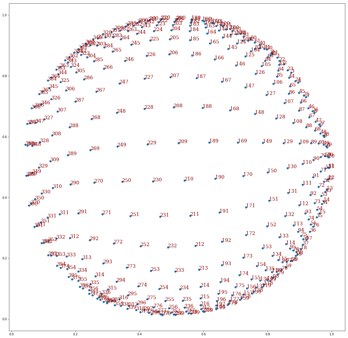
Furthermore, what’s really impressive with SOMs is that the original “topology” of the SOM, here the point lattice, is preserved:
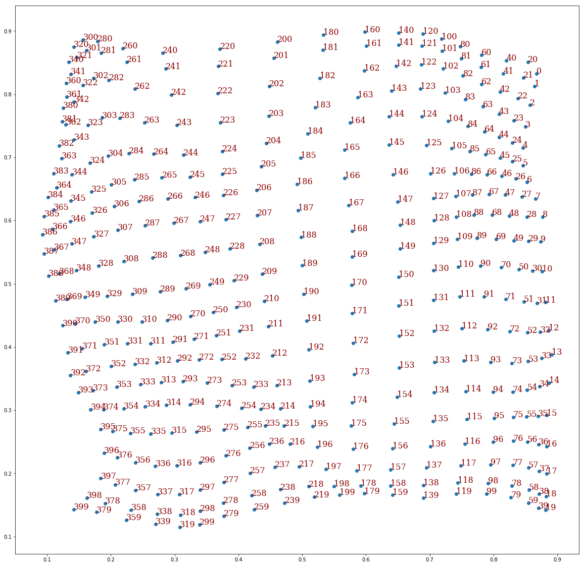
This huge image plots our feature vectors at the end of the training and adds on each of them the “ID” of the corresponding
cell on the SOM’s point lattice. If a cell has coordinates (y,x) on the lattice the ID is $20y+x$.
We see that here, the (0,0) cell corresponds to the right top corner of the square.
It’s very much as if the SOM was a piece of cloth physically matching the points it has been fed.
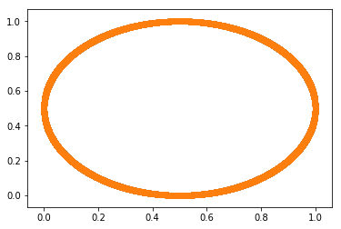
Inputing a circle
Let’s challenge our 2D SOM. We saw that we retrieved the point lattice structure at the end of training. Intuitively it was a good fit because our squared input data was more or less easily representable with this structure. Now, what if we fed the SOM with data that has nothing to do with a square ? For instance, the rim of a circle.
1
2
3
4
5
#Reference: https://stackoverflow.com/questions/8487893/generate-all-the-points-on-the-circumference-of-a-circle
def PointsInCircum(r,n=5000):
    return np.array([[math.cos(2*np.pi/n*x)*r+0.5,math.sin(2*np.pi/n*x)*r+0.5] for x in range(0,n+1)])

circle_data = PointsInCircum(0.5)
It gives, for instance, the following set of input points:
Let’s train the SOM with the same parameters:
1
2
3
4

    som_circle = SOM(20,20,2)
    frames_circle = []
    som_circle.train(circle_data,L0=0.8,lam=1e2,sigma0=10,frames=frames_circle)
It gives this final set of feature vectors:
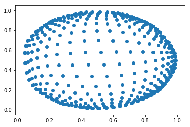
The SOM “imitated” the circle as it could!!
Here’s the whole training video:
And, again, the SOM’s point lattice topology was somehow preserved:
Therefore, whereas it seems impossible for the SOM to match the exact circumference of a circle, it fits it by expanding like a disc. Neat…
It even looks better than our square that was supposed to be a really good fit for the point lattice. However let’s take into account that we had data from inside the square during the training. Thus not all steps were informational in terms of shape because when an input data point already was inside the SOM area it would change almost nothing. It’s quite certain that redoing the square training but only with points on the border of the square would lead to “more visual” results.
Conversly, feeding input data points from all over a disc may lead to weird results.
Colors
We used 2D feature vectors in order to visualize the training of our SOM. In the same spirit, there’s a type of 3D features that can be visualized: colors.
However our approach is going to be a bit different. While we had a lot of data in the previous example we are going
to fed the SOM with only 3 colors. We’ll then plot the SOM with the colors on it which is straightforward when using
the plt.imshow matplotlib routine.
We first generates our random colors:
1
color_data = np.random.rand(3,3)
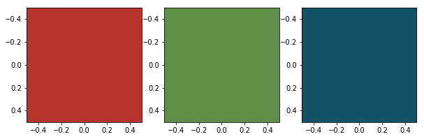
Then train the SOM:
1
2
3
som_color = SOM(40,40,3)
frames_color = []
som_color.train(color_data,L0=0.8,lam=1e2,sigma0=20,frames=frames_color)
At the end of the learning we get:
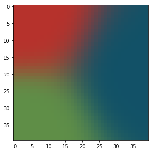
It looks very much like a Voronoï diagram. Three regions have been created, one for each color.
Here’s the video of the training:
In that example, the sigma(t) < 0.5 condition and the $\lambda = 10^2$ we chose have made
the learning quite long whereas the SOM stabilizes early (around 0.25s over 2.27m on the video).
What’s next ?
If you want to see an even more concrete example of how to use SOMs checkout a project I did on how to recognize apparels on pictures here.
References
Articles
Code
[SOM code]
[SOM notbook]
[SOM visualization]
Report
Websites
[1]: http://www.scholarpedia.org/article/Kohonen_network
[2]: http://cis.legacy.ics.tkk.fi/research/som-bibl/vol1_4.pdf
[3]: http://www.ai-junkie.com/ann/som/som1.html
[4]: https://github.com/alexhagen/jdc