About Free Energy

Introduction

Free energy is a concept which seems to be central in statistical physics, thermodynamics, chemistry and physical biology. More specifically, the idea that free energy is a quantity which systems naturally tend to minimize is very developed in those fields.

However, how can we build an intuition about the following textbook definition of free energy:

Where:

• $E$ is the energy (sometimes enthalpy $H$ is used instead of $E$)
• $T$ the temperature
• $S$ the entropy

To begin with, this expression of $G$ seems to be ill-typed because “energy” and “entropy” are not properties of the same kind of objects. Said differently, $E$ is the energy of what ? $S$ is the entropy of what ? Indeed, as presented in our article on entropy, entropy is a property of a probability distribution (or a random variable) while the energy $E$ seems to be the property of a state of a physical system. So how can we make sense of the expression of $G$ when $E$ and $S$ seem to be about very different things?

In this article, we answer that question by presenting a formalism of free energy with random variables. We’ll rewrite $G$ as being the property of a system state random variable $X$ together with an energetic valuation function $v$. We will write:

Where:

• $X$ is the random variable indicating in which state (microstate) our system is currently in
• $v:\Omega \to \mathbb{R}$ is a function indicating what is the energy of a given state $s\in\Omega$ ($\Omega$ is the set of all states)
• $\mathbb{E}[v(X)]$ is the expectation of $v(X)$, i.e. the average energy of the system with valuation $v$
• $\tau$ is a non-negative parameter called the ‘‘threshold’’
• $H(X)$ is the Shannon entropy of $X$ (not to be mistaken with some enthalpy $H$)

We intentionally use the term “threshold” instead of the term “temperature” because, in this mathematical model we don’t deal with units and physical scales.

Thanks to this formulation we’ll get some intuition on what minimizing $G$ means: finding the best compromise between stability (being in a low energy state) and “chaos” which is the natural ability of a system to explore all its possible states. With the theory of optimization we will be able to show that the probability distribution of $X$ which minimizes $G$ corresponds exactly to the Boltzmann distribution. Indeed, in this formalism, the principle of free energy minimization directly leads to the Boltzmann distribution and justifies why, in statistical physics, the probability for a system to be at a level of energy $E_i$ is given by:

Finally, throughout the article, we’ll illustrate this formalism on a concrete toy example of hybridization of two particles in a 1D-world.

Toy Model of Hybridization

Two Particles 1D-World

Figure 1. Three of the $N^2 + N$ states of the two particles 1D-world of size $N=5$.
The two particles can possibly bind if they are on the same cell.

Our toy model of hybridization is as follows: we take two distinct particles (a circle and a square in Figure 1 and 2) living in a disrcete, one dimensional, world composed of $N$ cells. These two particles can freely move to any cell of the world, in particular they can both be on the same cell (Figure 1, first and second rows). When they are on the same cell these two particles can “hybridize”, i.e. make a bond between themselves (Figure 1, third row).

Micro and Macro States

As shown in Figure 2, this system can be in $N^2+N$ states which we call microstates:

Figure 2. The $N^2 + N$ microstates of the system and its two macrostates: *bonded* or *not bonded*. Here, $N=5$.

These $N^2 + N$ microstates can be grouped in two distincts macrostates according to whether or not there is a bond between the particles or not. Macrostates are collections of microstates sharing a common property. Here we have two macrostates: bonded and not bonded.

Our System as a Random Variable

Let $X$ be the random variable indicating in which microstate the system is. The set of all microstates, $\Omega = \{ S_1, \ldots, S_{N^2 + N} \}$, is given in Figure 2. Formally, $X$ is the identity on $\Omega \to \Omega$.

The question we ask is: “What is the probability to be in a given microstate ?”. Equivalently: what is the distribution $p_X$ of the state variable $X$?

In order to answer this question we introduce the concept of energy of a state $S_i$.

Free Energy or the Fight Between Energy and Entropy

Some States are more Favored than Others

We are going to look at each of our microstate $S_i$ and state how favorable this state is. In other words, for each microstate, we are going to give a score encompassing how much our system favors this state with the intuition that, the more a state is favored the more likely is our system to end up in that state.

This score is the energy of the microstate. By convention energies are numbers in $\mathbb{R}$ and the lowest is the score, the more favored is the state. A microstate with energy $E=1000$ will be less more favored than a microstate with energy $E=-1000$. Formally, we are going to construct an energetic valuation function $v:\Omega \to \mathbb{R}$ by defining $v(S_i)$ for $1 \leq i \leq N+N^2$.

In our 1D-world, any microstate where the two particles are bonded will be considered as more favored – i.e having a lower energy – than any microstate where they are not bonded. Furthermore, in our model there is no reason to give a different energetic score to two microstates being in the same macrostate. Indeed, energetically speaking, nothing distinguishes microstates $1$ to $N^2$ (not bonded case) as well as nothing distinguishes microstates $N^2+1$ to $N^2+N$ (bonded case).

Hence we have:

In the following we take $E_{0} = 0$ as a reference energy. The value of $E_{1}$ (negative) will account for how intense is the bond between the two particles. For instance $E_{1} = -100$ will correspond to a situation where that bond is 10 time stronger than a scenario where $E_{1} = -10$. In a case like this one where energy refers to the intensity of a bond, the term enthalpy is often used instead of energy.

What is a Fair Distribution on Microstates?

Our goal is to construct $p_X = (p_1, \ldots, p_{N^2 + N})$, the probability distribution over microstates: $p_i$ is the probability that the system is in microstate $S_i$. In order to get there we must describe what is a good (or a fair) distribution over the microstates space.

For instance, would it be fair if $p_X$ was uniform, i.e all microstates are equally likely $p_i = \frac{1}{N^2 + N}$ ? No, because of the energetic argument. Indeed, microstates corresponding to the bonded macrostate are more favored by the system than not bonded microstates. Hence, our distribution $p_X$ must be biased in favor of the microstates in the bonded macrostate: $S_{N^2 + 1} \dots S_{N^2 + N}$.

Inversely, would it be fair if $p_X$ was concentrated over one particular microstate? For instance if we set $p_{N^2+1} = 1$? No, because of the entropic argument. The entropic argument accounts for the chaotic nature of microscopic systems: molecular agitation drives the system to explore its different possible configurations. Molecular agitation limits our ability to predict in which microstate the system is. This entropic effect, in physics, is proportional to the temperature. In our mathematical model, it will be proportional to the threshold.

Gibbs free energy will provide an answer to achieving a good compromise between the energetic and the entorpic argument.

Minimizing Free Energy: a Compromise between Energy and Entropy

Gibbs (or Helmholtz) free energy is a mathematical formalisation of the intuitive idea of a fight between energy and entropy in microscopic systems. We define it as follows:

With $\mathbb{E}[v(X)] = \sum_{i} v(S_i) p_i$, the weighted average energy, $\tau \geq 0$ a parameter called the threshold and $H(X)$ the Shannon entropy of $X$.

If we minimize $G(X,v)$, i.e. find the probability distribution $p_X$ which gives the smallest value of $G$, we achieve an interesting compromise. Indeed, we minimize the weighted average energy of the system while maximizing the corresponding entropy of the microstates distribution. Note that maximizing Shannon entropy matches the intuitive idea of the entropic argument since we maximize the lack of predictability of the random variable $X$ (see our article). The energetic argument is formalised by the idea of minimizing $\mathbb{E}[v(X)]$, the weighted average energy of our system.

The parameter $\tau$ allows us to linearly control the lack of predictability (or chaos) of the system. If $\tau = 0$, there is no chaos. Minimizing free energy will correspond to deterministically set the system to one of the most favorable state (less energy state). If $\tau = +\infty$, the system microstate is totally unpredictable: minimizing free energy will lead to the uniform distribution on microstates and the system is so unstable that the energetic argument does not hold anymore. In physics, the threshold $\tau$, up to the normalization constant $k_{B}$, corresponds to temperature. Temperature linearly controls the molecular agitation of the system which determines the ability of the system to explore its state space.

Experimental Solution to Free Energy Minimization

In the case of our 1D-world we can write some code in order to minimize $G(X,\nu)$. Free energy becomes:

With:

And with $q_0 = N^2 p_0$ and $q_1 = N p_{N^2+1}$ the probabilities of the macrostates bonded and not bonded (recall that $(p_1,\ldots,p_N^2,p_{N^2+1},\ldots,p_{N^2+N})$ is the probability distribution over microstates and the probability distribution of the variable $X$).

Note that we have made the implicit assumption that microstates with the same energy had the same probability (i.e. $p_1 = p_2 = \dots = p_{N^2}$ and $p_{N^2+1} = p_{N^2+2} = \dots = p_{N^2+N}$). This assumption will be confirmed later on with the calculus leading to Boltzmann distribution. As of right now, this assumption helps us writing a feasible optimization routine since we only have to optimize over $(q_0, q_1)$ and not the whole $(p_1,\ldots,p_N^2,p_{N^2+1},\ldots,p_{N^2+N})$.

The following code optimizes \(G(X,\nu)\) in our grid world context for different threshold conditions. You can play with this code interactively in this notebook.

1
2
3
4
5
6
7
8
9
10
11
12
13
14
15
16
17
18
19
20
21
22
23
24
25
26
27
28
29
30
31
32
33
34
35
36
37
38
39
40
41
42
43
44
45
import scipy.optimize as opt
from scipy.optimize import LinearConstraint
from scipy.special import xlogy

import scipy.stats as stats
import numpy as np
import matplotlib.pyplot as plt

plt.style.use('dark_background')

def entropy(proba_dist, world_weights):
    return -(xlogy(proba_dist[0],proba_dist[0]/world_weights[0]) + 
      xlogy(proba_dist[1],proba_dist[1]/world_weights[1]))
    
def free_energy(proba_dist, thresh, energies, world_weights):
    return proba_dist.dot(energies) - thresh*entropy(proba_dist, world_weights)

N_cells = 100

N_not_bounded = N_cells**2
N_bounded = N_cells

E_not_bounded=0
E_bounded=-1000

thresh_space = np.linspace(0,1000, 200)

proba_mat = []
for thresh in thresh_space:
    result = opt.minimize(free_energy, x0 = np.array([0.5,0.5]), 
             args = (thresh,
                     np.array([E_not_bounded, E_bounded]), 
                     np.array([N_not_bounded, N_bounded])), 
             constraints = LinearConstraint(np.array([1.0,1.0]), 1.0, 1.0))
    proba_mat.append(result.x)
proba_mat = np.array(proba_mat)

plt.figure(figsize=(10,5))
plt.plot(thresh_space, proba_mat[:,0], label="Proba Not Bounded")
plt.plot(thresh_space, proba_mat[:,1], label="Proba Bounded")
plt.legend()
plt.xlabel('Threshold')
plt.ylabel('Probability')
plt.title('Energy/Entropy Trade-off')
plt.show()

This code produces the following output:

Figure 3. Compromise between energy and entropy in the 1D-world with $N=100$

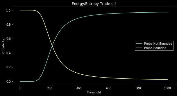
Figure 3 illustrates minimization of free energy depending on the threshold parameter. With this graph we realize the compromise made by free energy between energy and entropy. When the threshold is low, the energetic term wins and microstates with the lowest energy (i.e, in the bonded macrostate) are mainly favored ($q_{1} \simeq 1$). However, when the threshold gets very big, the entropic term wins and the solution to the minimization problem is the uniform distribution on microstates. In that case, since there are more microstates in the macrostate not bonded, the system behaves like a biased coin where $q_0 \simeq \frac{N^2}{N^2 + N}$ and $q_1 \simeq \frac{N}{N^2 + N} $.

In the notebook, you can experience the effect of other parameters on the overall result. You can for instance try modifying $E_{1}=E_{\text{bonded}}$ or $N$.

For instance, if you take $N=10$ instead of $N=100$, the difference between $\frac{N^2}{N^2 + N}$ and $\frac{N}{N^2 + N}$ becomes less important hence the not bonded case is less favored with $\tau$ big than when $N=100$:

Figure 4. Compromise between energy and entropy in the 1D-world N=$10$

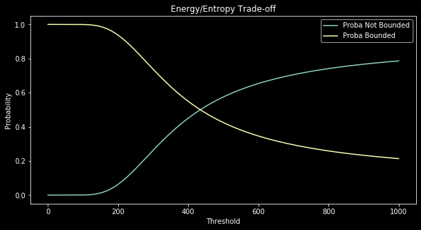
The melting point which is where the two curves meet in Figure 3 and 4 plays an important role in a wet lab experiment since, at it will appear with the next section, it allows to determine the value of $E_1-E_0$ (which is $E_1$ if we set $E_0=0$ as a reference value).

Analytical Solution to Free Energy Minimization: Boltzmann Distribution

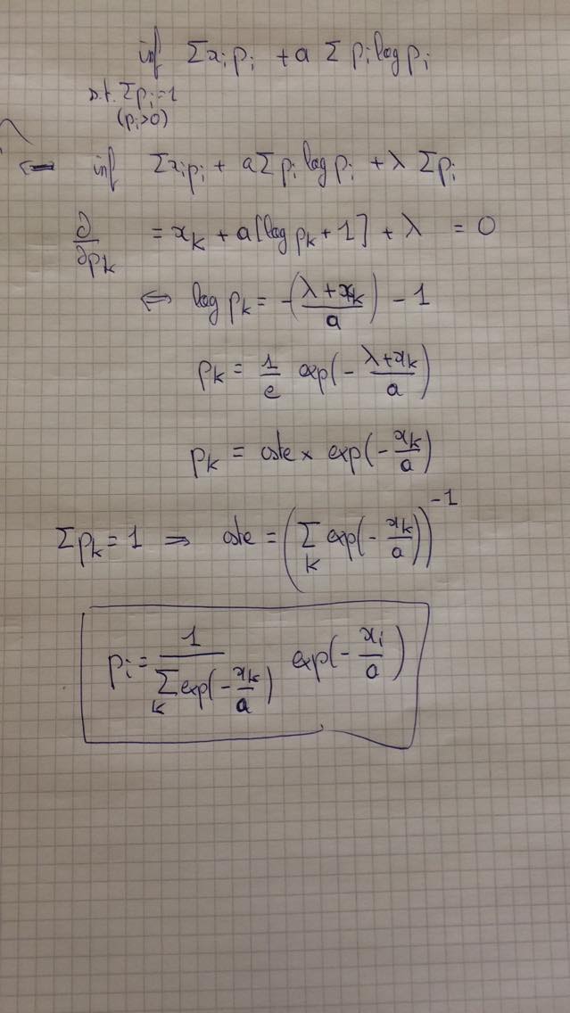
In the last section, we gave an experimental solution to the problem of Free Energy Minimization which is, given a $\nu$, find the microstates distribution $p_X$ which minimizes $G(X,v)$. In fact, thanks to the theory of Lagrange Multipliers this problem admits an analytical solution.

Indeed, the solution is uniquely given by:

With $Z=\sum_{i} e^{\nu(S_i)/\tau}$ a normalization factor also called partition function. If you are interested in how to solve this problem with Lagrange Multipliers please see this (thanks to Scott Pesme!).

Also, we can note that, as we assumed in the experimental section, microstates with same energies will have the same probabilities.

Finally, in the case of our grid world and according to Boltzmann distribution the probabilities of macrostates bonded and not bonded are given by:

The curves of Figure 3 and 4 should thus match the above expressions given by Boltzmann distribution.

The melting threshold $\tau^{\star}$, when $q_0=q_1=0.5$ is interesting because we get:

In a physical system, the threshold $\tau$ is in fact $k_{B}T$. Thus, if our toy model was physically meaningful for the hybridization of some particles and if we had an experimental way to determine the melting temperature $T^{\star}$, we could evaluate the energetics of the bonded state (assuming $E_0=0$ is a reference value) by:

In a real world experiment, $N$ would be replaced by some equivalent volumetric quantity.