About Shannon's Entropy
Introduction
The word and the concept of entropy might be familiar to you. It is usually associated with disorder, chaos, randomness, unpredictability. It originally came from physics where it was introduced in 1865 with the theory of thermodynamics. It was revisited in 1948 by the computer scientist Claude Shannon which interpreted it in terms of lack of information. This post aims at presenting you this informational point of view on entropy.
Entropy is at the root of Shannon’s Information Theory. You might never have heard of Information Theory but you use it every day!! Indeed, among others:
- It provides the mathematical tools for Data Compression such as, in practice: zip, jpeg, mp3, mp4, etc. Huge internet infrastructures such as YouTube or Facebook use them extensively to store data.
- It’s as the source of Error Correcting Codes that make possible the communication of data with possible loss on the way. Internet’s efficiency deeply depends on it as its communication channels are highly unreliable.
The first part of this post is purely informal and requires no particular background. In a second part we present a minimal formalization that leads to the construction of Shannon’s entropy.
An Intuitive Approach to Shannon’s Entropy
Random phenomenons
Entropy is a property of random phenomenons. More precisely, entropy is a property of the probability distribution of a random phenomenon.
A random phenomenon is any event of which outcome can be described by a probability distribution. For instance, the roll of a perfect dice can be seen as a random phenomenon with six possible outcomes (from “one” to “six”) with probability distribution $(1/6,1/6,1/6,1/6,1/6,1/6)$: each outcome is as likely to happen as any other. If I bias my dice in order to more frequently see the outcome “one” and never see neither “five” or “six”, I could end up with the following distribution: $(3/6,1/6,1/6,1/6,0,0)$.
In our case, a probability distribution is a finite set of non-negative numbers summing to one, we can think of them as percentages.
Weather Forecasts
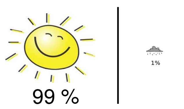
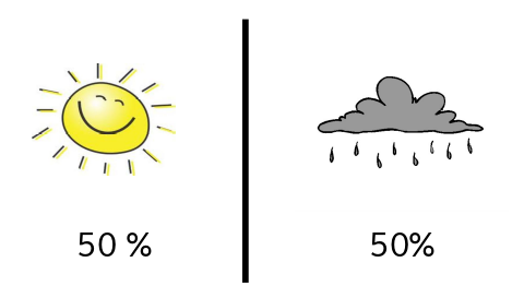
An other example of a random phenomenon is tomorrow’s weather: let say it’s either rainy or sunny. Now consider the two above forecasts. If you were to plan a hiking trip with your friends, which of the two forecasts would give you the most information ?
Very certainly the first one: you know you can go safely on your trip without taking any umbrella since it is so unlikely to rain. Similarly, if the forecast was 99% rainy, 1% sunny, you would know to definitely take an umbrella with you.
However, the second forecast is of very little help for you planning your trip. This forecast gives you the highest uncertainty about tomorrow’s weather: you have no idea weather it’s going to rain or not!
We could imagine a third forecast, for instance 30% sunny and 70% rainy, which does not convey as much information as the first forecast but which still gives better reasons to take an umbrella compared to the second forecast.
The intuition behind entropy
Entropy is exactly the metric which encompasses the above intuition. A probability distribution (a weather forecast in the above example), will have a high entropy if it gives you very little information about the outcome of the underlying random phenomenon. Conversly, it will have a low entropy if it gives the random phenomenon more determination.
In that sense, entropy measures the lack of information or uncertainty conveyed by a probability distribution on the outcome of a random phenomenon. To follow this intuition, the entropy of a random phenomenon with $k$ outcomes will be:
- Maximal if the random distribution is uniform: $(1/k,1/k, \dots, 1/k)$. For instance, an unbiased coin or dice.
- Minimal if the random distribution is deterministic that is, has one entry with probability one and all the others to zero. For instance, $(1,0,0,0,0,0)$ the probability distribution of a dice which has been biased to always output “one”.
Note that we expect entropy to be symmetric. Indeed, we consider to have as much information with a forecast 80% rainy, 20% sunny than with a forecast 20% rainy 80% sunny.
Mathematical formalism
Shannon entropy formula
Let $X$ be the random variable associated to a given random phenomenon (for instance $X$ is the variable “tomorrow’s weather”), and $p_X=(p_1,\dots,p_k)$ its distribution. Shannon’s entropy, $H(X)$ which satisfies the intuition developed in the above section is given by:
\[H(X) = \sum_{i=1}^k p_i \text{log}(1/p_i) = -\sum_{i=1}^k p_i \text{log}(p_i) \label{eq:shannon}\]Computer scientists will tend to choose the log in base two while physicists may prefer to use the log in base $e$. This choice changes nothing with respect to the intuitive interpretation of entropy. Indeed we have:
\[0 \leq H(X) \leq \text{log}(k)\]With $H(X) = 0$ if and only if $p_X$ is deterministic ($p_X$ of the form $(0,\dots,1,\dots,0)$) and $H(X) = \text{log}(k)$ if and only if $p_X$ is uniform $p_X=(1/k,\dots,1/k)$. Furthermore, the expression of Shannon’s entropy exhibits the symmetry we were expecting: take any permutation of $p_X$, you will get the same entropy.
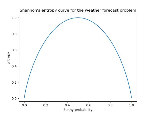
In the above graph, we plot $H(X)$ when there are only two outcomes, like in the weather forecast problem, $p_X = (p_\text{sunny},p_\text{rainy}) = (p_1,p_2)$. Because we have $p_2 = 1-p_1$ we can plot the whole in 2D. We notice the maximum at $p_1 = p_2 = 0.5$ and the minimum at $(p_1,p_2) = (0,1)$ and $(p_1,p_2) = (1,0)$ as expected. We also clearly see the symmetry in $p_1,p_2$.
Axiomatic fundations
We can legitimately ask the following question: where does the expression of Shannon’s entropy ($\ref{eq:shannon}$) comes from? More formally, from which axioms, this expression can be uniquely derived?
As highlighted in the different references at the end of this article, the answer to this question is not unique. We find in the litterature at least three different axiomatic approaches to the definition of entropy. None of them matches the intuition level on a straightforward way. However, the approach which might be the closest to our intuition might be Khinchin’s (Khinchin, 1957).
Khinchin gives four axioms to define $H$. Here are the first three axioms which are really close to our intuition on H:
- $H(X)$ should only depend on $p_X$
- If $X$ is a random variable with $k$ outcomes, $H(X)$ should be maximal when $p_X$ is uniform, that is when $p_X=(1/k,\dots,1/k)$
- If $X$ is such that $p_X = (p_1,\dots,p_k)$ and $Y$ such that $p_Y=(p_1,\dots,p_k,0,0,\dots,0)$ then $H(X) = H(Y)$
The fourth axiom would require too many details to be fully covered. We are going to give a weaker version which can more easily match our intuition. For the full details, refer to this course ([1]). The weaker version states that:
- If $X$ and $Y$ are two independent random variables then the entropy of their product $(X,Y)$ is given by:
Intuitively, this states that if $X$ and $Y$ dont share any information (knowing X doesn’t give you any information on Y and conversly) then their uncertainty sum up when you pair them together.
For instance, take $X$ tomorrow’s weather and $Y$ the outcome of a 6-faced dice you have on your desktop. It seems reasonable to say that $X$ and $Y$ are independent of each other. Then the variable $(X,Y)$ represents all the possible outcomes of this pair of phenomenon: (sunny, “one”), (sunny, “two”), (sunny, “three”) …, (rainy, “five”), (rainy, “six”). What equation $\ref{eq:sum}$ states is that the uncertainty of this pair of phenomenons is the sum of the uncertainty of the two individual phenomenons.
Why not. This requirement seems pretty reasonable. At least, our uncertainty on the pair of phenomenons depends on both phenomenons and is greater that the two individual uncertainties. Also, the transformation of a product into a sum guides our intuition to appreciate why the $\text{log}$ function is involved in the expression of Shannon’s entropy.
However, as mentionned earlier, this fourth axiom is too weak to lead uniquely to Shannon’s entropy. It gives a broader class of functions known as Rényi entropies:
\[H_{\alpha}(X) = \frac{1}{1-\alpha}\text{log}\sum_{i=1}^k p_i^\alpha\]With $\alpha \geq 0$. Shannon’s entropy is recovered when $\alpha = 1$: the limit of the above expression in $\alpha=1$ exists and is Shannon’s entropy.
Wrapping up
A random phenomenon, through its probability distribution, has an intrinsic property: entropy. Entropy measures the lack of knowledge (predictability) we have on this random phenomenon. It is a measure of uncertainty.
Different formalism all lead to the definition of Shannon’s entropy which meets our intuition with the principal characteristics of entropy:
- Entropy is maximal when the distribution is uniform, minimal when the distribution is deterministic
- Entropy is symmetric with respect to the probability distribution
- Entropy grows when two independent phenomenons are considered together
Shannon’s entropy naturally arises when notion as optimal compression or communication over a noisy channel are considered. It is at the root of Information Theory which is a crucial element of our understanding of communication processes both on the theoretical and practical point of view. Information theory introduces other very interesting quantities such as Kullback Leibler Divergence, Mutual Information* or Conditional Entropy.
We invite the curious reader to read an Information Theory course :) !
What about Physics?
Entropy is an important quantity in physics and chemistry, for instance in thermodynamic or statistical physics. So what is the link between this information theoretic point of view and physics?
Ask a physicist!!! (or look at our post on Free Energy.. )
References
[1], original link: https://www.stat.cmu.edu/~cshalizi/350/2008/lectures/06a/lecture-06a.pdf
[2], original link: https://arxiv.org/pdf/quant-ph/0511171.pdf
[3], original link: http://www.cs.tau.ac.il/~iftachh/Courses/Info/Fall15/Printouts/Lesson1_h.pdf